ST558-Project2
ST558 - Project 2
Li Wang & Bryan Bittner 2022-07-10
rmarkdown::render("Project2.Rmd",
                  output_format = "github_document",
                  output_file = "README.md",
                  output_options = list(html_preview= FALSE,toc=TRUE,toc_depth=2,toc_float=TRUE)
)
Load Packages
We will use the following packages:
library(rmarkdown)
library(httr)
library(jsonlite)
library(readr)
library(tidyverse)
library(lubridate)
library(knitr)
library(caret)
library(randomForest)
library(corrplot)
library(gbm)
Introduction
This online News Popularity Data Set summarizes a heterogeneous set of features about articles published by Mashable in a period of two years.
Our target variable is the shares variable(Number of shares ), and predict variables are the following:
- publishing_day: Day of the article published
- n_tokens_title: Number of words in the title
- n_tokens_content: Number of words in the content
- num_self_hrefs: Number of links to other articles published by Mashable
- num_imgs: Number of images
- num_videos: Number of videos
- average_token_length: Average length of the words in the content
- num_keywords: Number of keywords in the metadata
- kw_avg_min: Worst keyword (avg. shares)
- kw_avg_avg: Avg. keyword (avg. shares)
- self_reference_avg_shares: Avg. shares of referenced articles in Mashable
- LDA_04: Closeness to LDA topic 4
- global_subjectivity: ext subjectivity
- global_rate_positive_words: Rate of positive words in the content
- rate_positive_words: Rate of positive words among non-neutral tokens
- avg_positive_polarity: Avg. polarity of positive words
- min_positive_polarity: Min. polarity of positive words
- avg_negative_polarity: Avg. polarity of negative words
- max_negative_polarity: Max. polarity of negative words
- title_subjectivity: Title subjectivity
The purpose of our analysis is to predict the number of shares in social networks (popularity). In this project, we produce some basic summary statistics and plots about the training data, and fit a linear regression model and an ensemble tree-based model.
Data
Use a relative path to import the data.
newsData<-read_csv(file="../Datasets/OnlineNewsPopularity.csv",show_col_types = FALSE)
head(newsData)
## # A tibble: 6 × 61
##   url                timedelta n_tokens_title n_tokens_content n_unique_tokens n_non_stop_words n_non_stop_uniq… num_hrefs
##   <chr>                  <dbl>          <dbl>            <dbl>           <dbl>            <dbl>            <dbl>     <dbl>
## 1 http://mashable.c…       731             12              219           0.664             1.00            0.815         4
## 2 http://mashable.c…       731              9              255           0.605             1.00            0.792         3
## 3 http://mashable.c…       731              9              211           0.575             1.00            0.664         3
## 4 http://mashable.c…       731              9              531           0.504             1.00            0.666         9
## 5 http://mashable.c…       731             13             1072           0.416             1.00            0.541        19
## 6 http://mashable.c…       731             10              370           0.560             1.00            0.698         2
## # … with 53 more variables: num_self_hrefs <dbl>, num_imgs <dbl>, num_videos <dbl>, average_token_length <dbl>,
## #   num_keywords <dbl>, data_channel_is_lifestyle <dbl>, data_channel_is_entertainment <dbl>, data_channel_is_bus <dbl>,
## #   data_channel_is_socmed <dbl>, data_channel_is_tech <dbl>, data_channel_is_world <dbl>, kw_min_min <dbl>,
## #   kw_max_min <dbl>, kw_avg_min <dbl>, kw_min_max <dbl>, kw_max_max <dbl>, kw_avg_max <dbl>, kw_min_avg <dbl>,
## #   kw_max_avg <dbl>, kw_avg_avg <dbl>, self_reference_min_shares <dbl>, self_reference_max_shares <dbl>,
## #   self_reference_avg_sharess <dbl>, weekday_is_monday <dbl>, weekday_is_tuesday <dbl>, weekday_is_wednesday <dbl>,
## #   weekday_is_thursday <dbl>, weekday_is_friday <dbl>, weekday_is_saturday <dbl>, weekday_is_sunday <dbl>, …
Subset the data. If running the reports by an automated parameter driven process, the report will automatically use the parameter passed into this report. If running the report manually without a parameter, the data will subset to the ‘lifestyle’ news channel.
#Read the parameter being passed in to the automated report
if (params$columnNames != "") {
  paramColumnNameType<-params$columnNames
}else{
  paramColumnNameType<-"lifestyle"
}

columnName<-paste("data_channel_is_",paramColumnNameType,sep="")

#According to dplyr help, to refer to column names stored as string, use the '.data' pronoun.
#https://dplyr.tidyverse.org/reference/filter.html
newsDataSubset <- filter(newsData,.data[[columnName]] == 1)
Merging the weekdays columns channels as one single column named publishing_day.
# Merging the weekdays columns channels as one single column named publishing_day
newsDataSubset <- newsDataSubset %>%
  select(url, starts_with("weekday_is")) %>%
  pivot_longer(-url) %>%
  dplyr::filter(value > 0) %>%
  mutate(publishing_day = gsub("weekday_is_", "", name)) %>%
  left_join(newsDataSubset, by = "url") %>%
  select(-name, -starts_with("weekday_is_"))

# set the publishing_day as factor variable
newsDataSubset$publishing_day<- as.factor(newsDataSubset$publishing_day)
head(newsDataSubset)
## # A tibble: 6 × 56
##   url     value publishing_day timedelta n_tokens_title n_tokens_content n_unique_tokens n_non_stop_words n_non_stop_uniq…
##   <chr>   <dbl> <fct>              <dbl>          <dbl>            <dbl>           <dbl>            <dbl>            <dbl>
## 1 http:/…     1 monday               731              8              960           0.418             1.00            0.550
## 2 http:/…     1 monday               731             10              187           0.667             1.00            0.800
## 3 http:/…     1 monday               731             11              103           0.689             1.00            0.806
## 4 http:/…     1 monday               731             10              243           0.619             1.00            0.824
## 5 http:/…     1 monday               731              8              204           0.586             1.00            0.698
## 6 http:/…     1 monday               731             11              315           0.551             1.00            0.702
## # … with 47 more variables: num_hrefs <dbl>, num_self_hrefs <dbl>, num_imgs <dbl>, num_videos <dbl>,
## #   average_token_length <dbl>, num_keywords <dbl>, data_channel_is_lifestyle <dbl>, data_channel_is_entertainment <dbl>,
## #   data_channel_is_bus <dbl>, data_channel_is_socmed <dbl>, data_channel_is_tech <dbl>, data_channel_is_world <dbl>,
## #   kw_min_min <dbl>, kw_max_min <dbl>, kw_avg_min <dbl>, kw_min_max <dbl>, kw_max_max <dbl>, kw_avg_max <dbl>,
## #   kw_min_avg <dbl>, kw_max_avg <dbl>, kw_avg_avg <dbl>, self_reference_min_shares <dbl>,
## #   self_reference_max_shares <dbl>, self_reference_avg_sharess <dbl>, is_weekend <dbl>, LDA_00 <dbl>, LDA_01 <dbl>,
## #   LDA_02 <dbl>, LDA_03 <dbl>, LDA_04 <dbl>, global_subjectivity <dbl>, global_sentiment_polarity <dbl>, …
Here we drop some non-preditive variables: url,value,timedelta,data_channel_is_lifestyle, data_channel_is_entertainment,data_channel_is_bus, data_channel_is_socmed ,data_channel_is_tech,data_channel_is_world columns,is_weekend. They won’t contribute anything.
newsDataSubset<-newsDataSubset%>%select(-c(1,2,4,16:21,34))
newsDataSubset
## # A tibble: 2,099 × 46
##    publishing_day n_tokens_title n_tokens_content n_unique_tokens n_non_stop_words n_non_stop_unique_tokens num_hrefs
##    <fct>                   <dbl>            <dbl>           <dbl>            <dbl>                    <dbl>     <dbl>
##  1 monday                      8              960           0.418             1.00                    0.550        21
##  2 monday                     10              187           0.667             1.00                    0.800         7
##  3 monday                     11              103           0.689             1.00                    0.806         3
##  4 monday                     10              243           0.619             1.00                    0.824         1
##  5 monday                      8              204           0.586             1.00                    0.698         7
##  6 monday                     11              315           0.551             1.00                    0.702         4
##  7 monday                     10             1190           0.409             1.00                    0.561        25
##  8 monday                      6              374           0.641             1.00                    0.828         7
##  9 tuesday                    12              499           0.513             1.00                    0.662        14
## 10 wednesday                  11              223           0.662             1.00                    0.826         5
## # … with 2,089 more rows, and 39 more variables: num_self_hrefs <dbl>, num_imgs <dbl>, num_videos <dbl>,
## #   average_token_length <dbl>, num_keywords <dbl>, kw_min_min <dbl>, kw_max_min <dbl>, kw_avg_min <dbl>,
## #   kw_min_max <dbl>, kw_max_max <dbl>, kw_avg_max <dbl>, kw_min_avg <dbl>, kw_max_avg <dbl>, kw_avg_avg <dbl>,
## #   self_reference_min_shares <dbl>, self_reference_max_shares <dbl>, self_reference_avg_sharess <dbl>, LDA_00 <dbl>,
## #   LDA_01 <dbl>, LDA_02 <dbl>, LDA_03 <dbl>, LDA_04 <dbl>, global_subjectivity <dbl>, global_sentiment_polarity <dbl>,
## #   global_rate_positive_words <dbl>, global_rate_negative_words <dbl>, rate_positive_words <dbl>,
## #   rate_negative_words <dbl>, avg_positive_polarity <dbl>, min_positive_polarity <dbl>, max_positive_polarity <dbl>, …
Data Train/Test Split
Lets set up our Train/Test split. This will allow us to determine the model fit using a subset of data called Training, while saving the remainder of the data called Test to test our model predictions with.
set.seed(111)
train <- sample(1:nrow(newsDataSubset),size=nrow(newsDataSubset)*0.7)
test <- dplyr::setdiff(1:nrow(newsDataSubset),train)

newsDataSubsetTrain <- newsDataSubset[train,]
newsDataSubsetTest <- newsDataSubset[test,]
Summarizations
Data structure and basic summary statistics
Start with the data structure and basic summary statistics for the ‘shares’ field.
# data structure
str(newsDataSubsetTrain)
## tibble [1,469 × 46] (S3: tbl_df/tbl/data.frame)
##  $ publishing_day              : Factor w/ 7 levels "friday","monday",..: 1 5 1 6 5 4 6 5 5 7 ...
##  $ n_tokens_title              : num [1:1469] 13 8 14 8 11 11 13 9 10 12 ...
##  $ n_tokens_content            : num [1:1469] 776 1331 879 762 743 ...
##  $ n_unique_tokens             : num [1:1469] 0.499 0.419 0.419 0.375 0.532 ...
##  $ n_non_stop_words            : num [1:1469] 1 1 1 1 1 ...
##  $ n_non_stop_unique_tokens    : num [1:1469] 0.699 0.612 0.584 0.497 0.713 ...
##  $ num_hrefs                   : num [1:1469] 4 3 19 11 9 22 10 11 10 12 ...
##  $ num_self_hrefs              : num [1:1469] 2 0 4 2 0 2 5 3 3 1 ...
##  $ num_imgs                    : num [1:1469] 1 1 12 1 1 0 0 4 0 2 ...
##  $ num_videos                  : num [1:1469] 0 0 0 0 0 0 0 1 0 0 ...
##  $ average_token_length        : num [1:1469] 4.63 4.72 4.54 4.9 4.75 ...
##  $ num_keywords                : num [1:1469] 5 7 9 8 5 10 10 9 7 8 ...
##  $ kw_min_min                  : num [1:1469] -1 4 217 4 -1 -1 217 -1 4 -1 ...
##  $ kw_max_min                  : num [1:1469] 1600 1400 456 309 566 728 1400 690 2100 1000 ...
##  $ kw_avg_min                  : num [1:1469] 319 346 344 132 113 ...
##  $ kw_min_max                  : num [1:1469] 8100 24500 0 0 11600 39700 0 0 0 0 ...
##  $ kw_max_max                  : num [1:1469] 843300 843300 69100 843300 843300 ...
##  $ kw_avg_max                  : num [1:1469] 407740 209814 25289 153025 341800 ...
##  $ kw_min_avg                  : num [1:1469] 2488 2959 0 0 3397 ...
##  $ kw_max_avg                  : num [1:1469] 4640 10290 3073 4638 5972 ...
##  $ kw_avg_avg                  : num [1:1469] 3714 4967 2379 2946 4232 ...
##  $ self_reference_min_shares   : num [1:1469] 9800 0 11000 5200 0 2000 2300 1400 2900 2200 ...
##  $ self_reference_max_shares   : num [1:1469] 9800 0 11000 5200 0 2000 3400 24000 2900 2200 ...
##  $ self_reference_avg_sharess  : num [1:1469] 9800 0 11000 5200 0 ...
##  $ LDA_00                      : num [1:1469] 0.0408 0.0289 0.0226 0.0255 0.3398 ...
##  $ LDA_01                      : num [1:1469] 0.04 0.0287 0.0223 0.025 0.04 ...
##  $ LDA_02                      : num [1:1469] 0.2609 0.0286 0.0223 0.1508 0.0401 ...
##  $ LDA_03                      : num [1:1469] 0.2628 0.0286 0.2491 0.0251 0.0401 ...
##  $ LDA_04                      : num [1:1469] 0.396 0.885 0.684 0.774 0.54 ...
##  $ global_subjectivity         : num [1:1469] 0.424 0.386 0.42 0.378 0.388 ...
##  $ global_sentiment_polarity   : num [1:1469] 0.1147 0.1208 0.1898 0.0835 0.0744 ...
##  $ global_rate_positive_words  : num [1:1469] 0.0464 0.0331 0.0512 0.0315 0.0458 ...
##  $ global_rate_negative_words  : num [1:1469] 0.0193 0.0143 0.0171 0.021 0.0162 ...
##  $ rate_positive_words         : num [1:1469] 0.706 0.698 0.75 0.6 0.739 ...
##  $ rate_negative_words         : num [1:1469] 0.294 0.302 0.25 0.4 0.261 ...
##  $ avg_positive_polarity       : num [1:1469] 0.301 0.42 0.357 0.281 0.294 ...
##  $ min_positive_polarity       : num [1:1469] 0.0333 0.0333 0.1 0.0625 0.0625 ...
##  $ max_positive_polarity       : num [1:1469] 0.6 1 0.8 1 0.6 0.5 0.6 0.8 0.8 0.8 ...
##  $ avg_negative_polarity       : num [1:1469] -0.259 -0.25 -0.161 -0.144 -0.267 ...
##  $ min_negative_polarity       : num [1:1469] -1 -0.5 -0.8 -0.4 -0.8 -0.6 -0.8 -0.5 0 -0.8 ...
##  $ max_negative_polarity       : num [1:1469] -0.1 -0.125 -0.05 -0.05 -0.025 -0.3 -0.1 -0.05 0 -0.05 ...
##  $ title_subjectivity          : num [1:1469] 0 1 0.447 0 0.527 ...
##  $ title_sentiment_polarity    : num [1:1469] 0 0 0.253 0 -0.132 ...
##  $ abs_title_subjectivity      : num [1:1469] 0.5 0.5 0.0533 0.5 0.0273 ...
##  $ abs_title_sentiment_polarity: num [1:1469] 0 0 0.253 0 0.132 ...
##  $ shares                      : num [1:1469] 750 5100 3600 987 2600 1800 3700 2800 3400 1200 ...
# data summary
summary(newsDataSubsetTrain$shares)
##    Min. 1st Qu.  Median    Mean 3rd Qu.    Max.
##      28    1100    1600    3677    3200  208300
Now lets show the Mean, Median, Variance, and Standard Deviation. Notice the Variance and Standard Deviation are both extremely high. This might be something we will have to investigate further.
newsDataSubsetTrain %>% summarise(avg = mean(shares), med = median(shares), var = var(shares), sd = sd(shares))
## # A tibble: 1 × 4
##     avg   med       var    sd
##   <dbl> <dbl>     <dbl> <dbl>
## 1 3677.  1600 87380046. 9348.
Looking at the different columns in the dataset, there are two that stand out. Generally speaking, people probably aren’t going to look at articles that don’t have images or videos. Here are the summary stats for the articles grouped on the number of images in the article.
newsDataSubsetTrain %>% group_by(num_imgs) %>%
summarise(avg = mean(shares), med = median(shares), var = var(shares), sd = sd(shares))
## # A tibble: 39 × 5
##    num_imgs   avg   med       var    sd
##       <dbl> <dbl> <dbl>     <dbl> <dbl>
##  1        0 3251.  1700 23231753. 4820.
##  2        1 3469.  1500 89161464. 9443.
##  3        2 3653.  1500 99053188. 9953.
##  4        3 3086.  2050  9118448. 3020.
##  5        4 1867.  1200  2769069. 1664.
##  6        5 4640.  1800 84775414. 9207.
##  7        6 2960.  1500 26086991. 5108.
##  8        7 3293.  2300  5881784. 2425.
##  9        8 3106.  1850 15019514. 3876.
## 10        9 4285.  2250 42337039. 6507.
## # … with 29 more rows
As we can see from the above table, the number of shares tend to increase as the number of images increases. Therefore, the number of images variable affects shares, and we will keep this variable.
Here are the summary stats for articles with videos.
newsDataSubsetTrain %>% group_by(num_videos) %>%
summarise(avg = mean(shares), med = median(shares), var = var(shares), sd = sd(shares))
## # A tibble: 16 × 5
##    num_videos     avg    med        var     sd
##         <dbl>   <dbl>  <dbl>      <dbl>  <dbl>
##  1          0   3534.   1600  71966935.  8483.
##  2          1   3671.   1700  30614286.  5533.
##  3          2   2361.   1700   4504196.  2122.
##  4          3   3589.   1600  38755051.  6225.
##  5          4   6667.   2000  66743333.  8170.
##  6          5   8200.   1500 183997950. 13565.
##  7          6   6950    6950    245000    495.
##  8          7   9033    7050  99351823.  9968.
##  9          8    833     833        NA     NA
## 10          9   1100    1100        NA     NA
## 11         10   1699.   1300   1109348.  1053.
## 12         11   2833.   3100    303333.   551.
## 13         12   4400    4400   8000000   2828.
## 14         15 196700  196700        NA     NA
## 15         28    660     660        NA     NA
## 16         50    932     932        NA     NA
As we can see from the above table, number of shares tend to increase as the number of videos increases. Therefore, the number of videos variable affects shares, and we will keep this variable.
Plots
A plot with the number of shares on the y-axis and number of words in the title (n_tokens_title) on the x-axis is created:
g <- ggplot(newsDataSubsetTrain, aes(x = n_tokens_title, y = shares))
g + geom_point()+labs(title = "Plot of shares VS n_tokens_title")
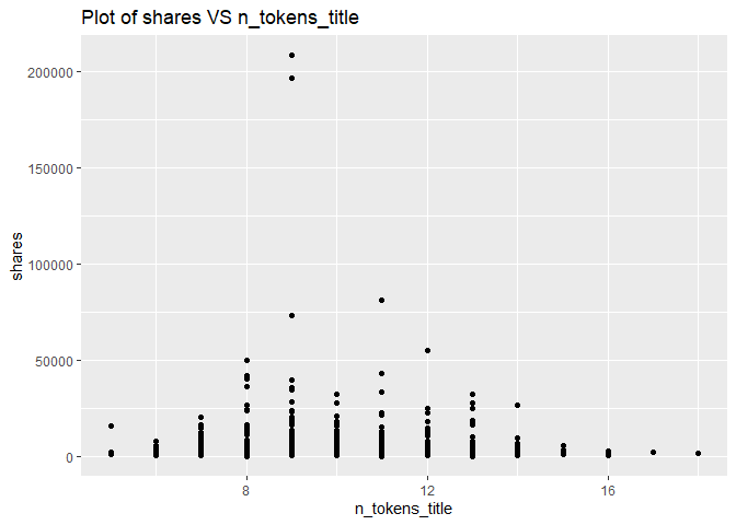
The number of shares will vary depending on on the channel type. But there is clearly a relationship between the number of words in the title and the number of shares. Therefore, the number of words in the title affects shares, and we will keep n_tokens_title variable.
A plot with the number of shares on the y-axis and publishing day (publishing_day) on the x-axis is created:
g <- ggplot(newsDataSubsetTrain, aes(x = publishing_day, y = shares))
g + geom_point()+labs(title = "Plot of shares VS publishing_day")
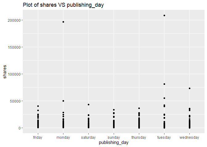
Looking at the plot, some of the days will have a higher number of shares and some of the days will have a lower number of shares. The days with the higher shares will vary depending on the channel. For example, it makes sense that some of the business related channels have a higher share rate during the work week than the weekend. Therefore, the publishing_day affects shares, and we will keep publishing_day.
A plot with the number of shares on the y-axis and rate of positive words (rate_positive_words) on the x-axis is created:
g <- ggplot(newsDataSubsetTrain, aes(x = rate_positive_words, y = shares))
g + geom_point()+labs(title = "Plot of shares VS rate_positive_words")
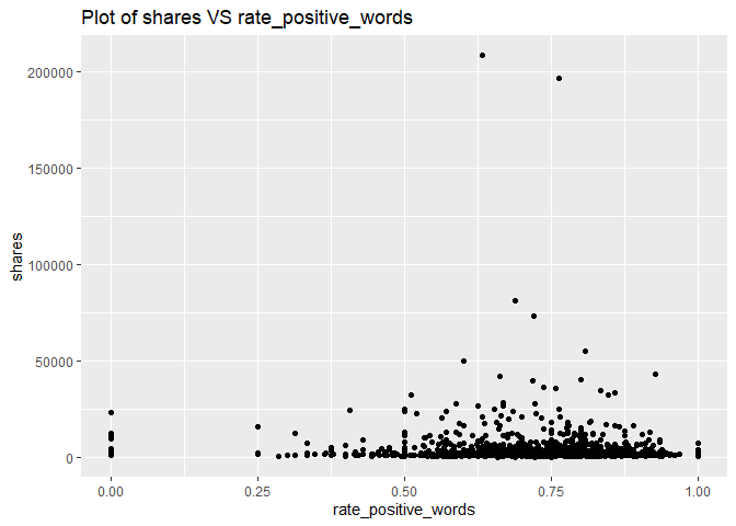
Looking across the plots for each of the channels, there is a correlation between using positive words and a higher share number. Therefore, the variable rate_positive_words effects shares, and we will keep this variable.
A plot with the number of shares on the y-axis and number of words in the content (n_tokens_content) on the x-axis is created:
g <- ggplot(newsDataSubsetTrain, aes(x = n_tokens_content, y = shares))
g + geom_point()+labs(title = "Plot of shares VS n_tokens_content")
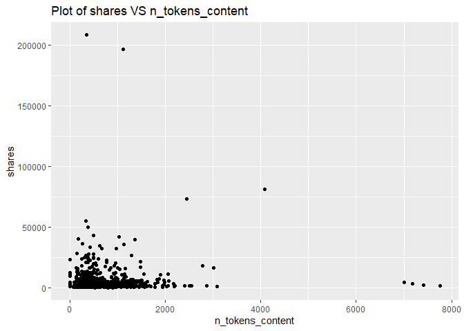
For each of the channel types, it is easy to see that the number of shares will decrease as the number of words in the article increases. For most channel types, the highest shares are with the articles that have less than 2000 words. Therefore, the variable n_tokens_content effects shares, and we will keep this variable.
A plot with the number of shares on the y-axis and average word length (average_token_length) on the x-axis is created:
g <- ggplot(newsDataSubsetTrain, aes(x = average_token_length, y = shares))
g + geom_point()+labs(title = "Plot of shares VS average_token_length")
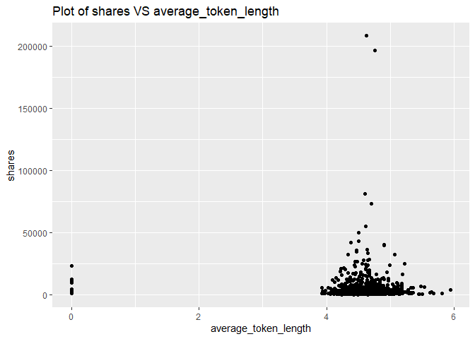
From the above plot, we can see that the most shares contain 4-6 length words. Therefore, the variable average_token_length effects shares, and we will keep this variable.
Correlation matrix plot is generated:
newsDataSubsetTrain1<-select(newsDataSubsetTrain,-publishing_day)
corr=cor(newsDataSubsetTrain1, method = c("spearman"))
corrplot(corr,tl.cex=0.5)
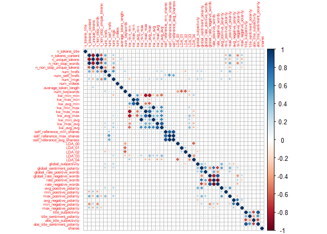
By the above correlation matrix plot, we can see these variables are strongly correlated:
- title_subjectivity, abs_title_sentiment_polarity, abs_title_subjectivity, title_sentiment_polarity
- avg_negative_polarity, min_negative_polarity
- max_positive_polarity, avg_positive_polarity
- global_rate_negative_words, rate_negative_words,rate_positive_words
- global_sentiment_polarity, rate_negative_words, rate_positive_words
- LDA_03,LDA_04
- LDA_00,LDA_04
- self_reference_max_shares, self_reference_avg_shares, self_reference_min_shares
- kw_max_avg, kw_avg_avg
- kw_min_avg,kw_avg_avg,kw_min_max
- kw_avg_max,kw_avg_avg,kw_max_max
- kw_avg_min,kw_avg_max
- kw_max_min,kw_avg_min,kw_min_min
- kw_min_min,kw_avg_max
- num_keywords,LDA_01
- num_keywords,LDA_02
- num_hrefs, num_imgs
- n_non_stop_unique_tokens, num_imgs
- n_non_stop_words, n_non_stop_unique_tokens
- n_unique_tokens,n_non_stop_unique_tokens
- n_unique_tokens, n_non_stop_words, n_tokens_content
- n_tokens_content, n_non_stop_unique_tokens
- n_tokens_content, num_hrefs
These are strongly correlated which makes us to assume that these features are so linearly dependent that any one of the strong correlated feature can be used and excluding the other features with high correlation.
Feature selection
Let’s do feature selection:
newsDataSubsetTrain2<-select(newsDataSubsetTrain,-abs_title_sentiment_polarity, -abs_title_subjectivity, -title_sentiment_polarity,-min_negative_polarity,-max_positive_polarity,-rate_negative_words,-global_rate_negative_words,-global_sentiment_polarity,-LDA_03,-LDA_00,-self_reference_max_shares,-self_reference_min_shares,-kw_max_avg,-kw_min_avg,-kw_min_max,-kw_avg_max,-kw_max_max,-kw_max_min,-kw_min_min,-LDA_01,-LDA_02,-num_hrefs,-n_non_stop_unique_tokens,-n_unique_tokens,-n_non_stop_words)

newsDataSubsetTest2<-select(newsDataSubsetTrain,-abs_title_sentiment_polarity, -abs_title_subjectivity, -title_sentiment_polarity,-min_negative_polarity,-max_positive_polarity,-rate_negative_words,-global_rate_negative_words,-global_sentiment_polarity,-LDA_03,-LDA_00,-self_reference_max_shares,-self_reference_min_shares,-kw_max_avg,-kw_min_avg,-kw_min_max,-kw_avg_max,-kw_max_max,-kw_max_min,-kw_min_min,-LDA_01,-LDA_02,-num_hrefs,-n_non_stop_unique_tokens,-n_unique_tokens,-n_non_stop_words)
Modeling
Linear Regression Model
A Linear Regression Model is the first model type we will look at. These models are an intuitive way to investigate the linear relation between multiple variables. These models make the estimation procedure simple and easy to understand. Linear Regression models can come in all different shapes and sizes and can be used to model more than just a straight linear relationship. Regression models can be modified with interactive and or higher order terms that will conform to a more complex relationship.
For the first linear model example, we can try a model using just the “num_imgs” and “num_videos” as our predictors.
set.seed(111)
#Fit a  multiple linear regression model using just the "num_imgs" and "num_videos" as our predictors.
mlrFit <- train(shares ~ num_imgs + num_videos,
                data = newsDataSubsetTrain2,
                method="lm",
                trControl=trainControl(method="cv",number=5))
mlrFit
## Linear Regression
##
## 1469 samples
##    2 predictor
##
## No pre-processing
## Resampling: Cross-Validated (5 fold)
## Summary of sample sizes: 1176, 1175, 1175, 1175, 1175
## Resampling results:
##
##   RMSE      Rsquared     MAE
##   8654.134  0.006868955  3338.509
##
## Tuning parameter 'intercept' was held constant at a value of TRUE
Next we can try a linear model using all of the fields as a predictor variables.
#Fit a  multiple linear regression model using all of the fields as a predictor variables.
set.seed(111)
mlrAllFit <- train(shares ~ .,
                data = newsDataSubsetTrain2,
                method="lm",
                trControl=trainControl(method="cv",number=5))
mlrAllFit
## Linear Regression
##
## 1469 samples
##   20 predictor
##
## No pre-processing
## Resampling: Cross-Validated (5 fold)
## Summary of sample sizes: 1176, 1175, 1175, 1175, 1175
## Resampling results:
##
##   RMSE      Rsquared     MAE
##   8766.142  0.008764755  3435.973
##
## Tuning parameter 'intercept' was held constant at a value of TRUE
Try a model using just the num_imgs + num_videos + kw_avg_avg + num_imgs*kw_avg_avg as our predictors.
set.seed(111)
#Fit a  multiple linear regression model with num_imgs + num_videos + kw_avg_avg + num_imgs*kw_avg_avg.
mlrInteractionFit <- train(shares ~ num_imgs + num_videos + kw_avg_avg + num_imgs*kw_avg_avg,
                data = newsDataSubsetTrain2,
                method="lm",
                trControl=trainControl(method="cv",number=5))
mlrInteractionFit
## Linear Regression
##
## 1469 samples
##    3 predictor
##
## No pre-processing
## Resampling: Cross-Validated (5 fold)
## Summary of sample sizes: 1176, 1175, 1175, 1175, 1175
## Resampling results:
##
##   RMSE      Rsquared    MAE
##   8629.451  0.03062777  3291.096
##
## Tuning parameter 'intercept' was held constant at a value of TRUE
Random Forest Model
The Random Forest Model is an example of an ensemble based model. Instead of traditional decision trees, ensemble methods average across the tree. This will greatly increase our prediction power, but it will come at the expense of the easy interpretation from traditional decision trees. The Random Forest based model will not use all available predictors. Instead it will take a random subset of the predictors for each tree fit and calculate the model fit for that subset. It will repeat the process a pre-determined number of times and automatically pick the best predictors for the model. This will end up creating a reduction in the overall model variance.
set.seed(111)
randomForestFit <- train(shares ~ .,
                         data = newsDataSubsetTrain2,
                         method="rf",
                         preProcess=c("center","scale"),
                         trControl=trainControl(method="cv",number=5),
                         tuneGrid=data.frame(mtry=ncol(newsDataSubsetTrain)/3))
randomForestFit
## Random Forest
##
## 1469 samples
##   20 predictor
##
## Pre-processing: centered (25), scaled (25)
## Resampling: Cross-Validated (5 fold)
## Summary of sample sizes: 1176, 1175, 1175, 1175, 1175
## Resampling results:
##
##   RMSE      Rsquared    MAE
##   9524.759  0.00306765  3817.129
##
## Tuning parameter 'mtry' was held constant at a value of 15.33333
Boosted Tree Model
Boosted Regression Tree (BRT) models are a combination of two techniques: decision tree algorithms and boosting methods. It repeatedly fits many decision trees to improve the accuracy of the model.
Boosted Regression Tree uses the boosting method in which the input data are weighted in subsequent trees. The weights are applied in such a way that data that was poorly modelled by previous trees has a higher probability of being selected in the new tree. This means that after the first tree is fitted the model will take into account the error in the prediction of that tree to fit the next tree, and so on. By taking into account the fit of previous trees that are built, the model continuously tries to improve its accuracy. This sequential approach is unique to boosting.
set.seed(111)
BoostedTreeFit <- train(shares ~ .,
                         data = newsDataSubsetTrain2,
                         distribution = "gaussian",
                         method="gbm",
                         trControl=trainControl(method="cv",number=5),
                         verbose = FALSE)
BoostedTreeFit
## Stochastic Gradient Boosting
##
## 1469 samples
##   20 predictor
##
## No pre-processing
## Resampling: Cross-Validated (5 fold)
## Summary of sample sizes: 1176, 1175, 1175, 1175, 1175
## Resampling results across tuning parameters:
##
##   interaction.depth  n.trees  RMSE      Rsquared     MAE
##   1                   50      8795.865  0.010744808  3366.154
##   1                  100      8812.067  0.009141891  3385.138
##   1                  150      8905.616  0.009836261  3437.492
##   2                   50      8830.359  0.009322874  3416.717
##   2                  100      8962.216  0.006257919  3463.981
##   2                  150      9052.275  0.002712680  3507.443
##   3                   50      8864.338  0.011828246  3413.643
##   3                  100      9026.561  0.007730813  3543.420
##   3                  150      9114.531  0.008093483  3588.768
##
## Tuning parameter 'shrinkage' was held constant at a value of 0.1
## Tuning parameter 'n.minobsinnode' was held constant at
##  a value of 10
## RMSE was used to select the optimal model using the smallest value.
## The final values used for the model were n.trees = 50, interaction.depth = 1, shrinkage = 0.1 and n.minobsinnode = 10.
Comparison
All the models are compared by RMSE on the test set
set.seed(111)
#compute RMSE of MlrFit
mlrFitPred <- predict(mlrFit, newdata = newsDataSubsetTest2)
MlrFit<-postResample(mlrFitPred, newsDataSubsetTest2$shares)
MlrFit.RMSE<-MlrFit[1]

#compute RMSE of MlrAllFit
MlrAllFitPred <- predict(mlrAllFit, newdata = newsDataSubsetTest2)
MlrAllFit<-postResample(MlrAllFitPred, newsDataSubsetTest2$shares)
MlrAllFit.RMSE<-MlrAllFit[1]

#compute RMSE of MlrInterFit
mlrInteractionFitPred <- predict(mlrInteractionFit, newdata = newsDataSubsetTest2)
MlrInterFit<-postResample(mlrInteractionFitPred, newsDataSubsetTest2$shares)
MlrInterFit.RMSE<-MlrInterFit[1]

#compute RMSE of RandomForest
ForestPred <- predict(randomForestFit, newdata = newsDataSubsetTest2)
RandomForest<-postResample(ForestPred, newsDataSubsetTest2$shares)
RandomForest.RMSE<-RandomForest[1]

#compute RMSE of BoostedTree
BoostPred <- predict(BoostedTreeFit, newdata = newsDataSubsetTest2)
BoostedTree<-postResample(BoostPred, newsDataSubsetTest2$shares)
BoostedTree.RMSE<-BoostedTree[1]

#Compare Root MSE values
c(MlrFit=MlrFit.RMSE,MlrAllFit=MlrAllFit.RMSE,MlrInterFit=MlrInterFit.RMSE,RandomForest=RandomForest.RMSE,BoostedTree=BoostedTree.RMSE)
##       MlrFit.RMSE    MlrAllFit.RMSE  MlrInterFit.RMSE RandomForest.RMSE  BoostedTree.RMSE
##          9285.358          9187.197          9214.330          5403.120          9059.082
From the above compare, we can see the smallest RMSE is 5403.120 which belong to RandomForest. Therefore, we will choose the Random Forest Model.
Automation
Below is a chuck of code that can be used to automate the reports. In order to automate this project, the first thing we do is build a set of parameters. These parameters match up with the column names from the full news dataset. The program with read the parameter and subset the data down to only values with the specified news channel name that is in the parameter.
To automate the project for all of the different news channels, simply execute the code chunk below directly to the console. Separate .md files will then be created for each news channel type.
#Add column names
columnNames <- data.frame("lifestyle","entertainment","bus","socmed","tech","world")

#Create filenames
output_file<-paste0(columnNames,".md")

#create a list for each column name
params = lapply(columnNames, FUN = function(x){list(columnNames = x)})

#put into a data frame
reports<-tibble(output_file,params)

#Render Code
apply(reports, MARGIN=1,FUN=function(x)
  {
    rmarkdown::render(input="Project2.Rmd",
    output_format="github_document",
    output_file=x[[1]],
    params=x[[2]],
    output_options = list(html_preview= FALSE,toc=TRUE,toc_depth=2,toc_float=TRUE)
    )
  }
)